Reflectors should be your second nature

Reflectors are a class of matrices that are not introduced in all linear algebra textbooks. However, the book of Carl D. Meyer uses this class of matrices heavily for various fundamental results. Indeed, the book uses reflectors for theoretical reasons, such as proving the existence of fundamental transformations like SVD, QR, Triangulation, or Hessenberg decompositions (more to come below), as well as applications, such as the implementation of the QR algorithm via the Householder transformation or solution of large-scale linear systems with Krylov methods (i.e., Lanczos’ Tridiagonalization algorithm or GMRES). A more comprehensive summary will be given by the end of the article, but hopefully you’re already excited.

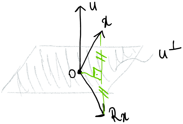
Elementary reflectors are a class of orthogonal matrices that are constructed from a vector $u$ with $||u||=1$ as (see p324 of Meyer)
$$
R = I-2uu^*.
$$

The function of a reflector about the complementary orthogonal subspace of $u$, namely $u^\perp$, is illustrated below.

It is somewhat curious that this relatively simple operator can form the foundation of so many important results in linear algebra. Below we try to uncover what are the properties that make this operator so special and useful.

Firstly, simple calculations reveal that all elementary reflectors have the property
$$
R = R^\star = R^{-1}.
$$
That is, elementary reflectors are involutory ($R^2=I$) as well as being orthogonal. The second key property of reflectors is that, for any given real vector $x$, we can find a reflector $R$ such that
$$
Rx = ||x||e_1 = \begin{pmatrix}||x|| \\0 \\0 \\ \vdots \\ 0\end{pmatrix}.
$$

The last but certainly not least property of reflectors is that if $R$ is an elementary reflector, the matrix
$$
\begin{pmatrix}I & 0 \\ 0 & R\end{pmatrix}
$$
is also an elementary reflector. You’ll see that the last two properties together are the key ingredient of the deflate-and-conquer strategy defined below.

The reflector trick: Deflate-and-Conquer

The deflate-and-conquer strategy illustrated below is the primary mechanism behind the many factorizations (QR, Schur, SVD, Hessenberg, …) based on elementary reflectors. The precise implementation depends on the desired transformation, but the in broad strokes, the strategy below remains the same.

We start from an $n\times n$ matrix. Then we process the first column; using an appropriately designed reflector, we make everything below the first entry of the column zero. Then we deflate the problem: we focus on the $n-1\times n-1$ matrix on the bottom right of the original matrix, and repeat what we did on this submatrix. We proceed this way until the last (i.e., $1\times 1$-sized) bottom-right submatrix.

The property of elementary reflectors that allows us to use this strategy is the second one listed above. Suppose that we want to compute the QR factors of matrix $A_{n\times n}$ (of rank $n$ — for clarity) whose first column is $a_1$. Then we construct a reflector $R_1$ such that
$$
R_1 a_1 = ||a_1|| e_1.
$$
It is easy to see that $R_1 A$ will produce a matrix whose first column contains zeroes except in its first entry, which is $||a_1||$:
$$
R_1 A_1 = \begin{pmatrix}||a_1|| & t_1^T \\ 0 & A_2\end{pmatrix}.
$$
Now we repeat the same thing on $A_2$; we find another elementary reflector $R_2$ such that the first column of the product $R_2 A_2$ is non-zero in its first entry and zero elsewhere. We continue in this way, producing a series of matrices $R_1, R_2, \dots, R_{n-1}$. Notice that none of these reflectors will be of the same size, since the deflation implies that these matrices will be respectively of size $n\times n$, $(n-1)\times (n-1)$, $(n-2)\times (n-2)$, $\dots$, $2\times 2$. This naturally raises the question of how we’ll integrate these matrices into a QR factorization.

Enter the third property listed above. Define $\hat R_k$ as
$$
\hat R_k = \begin{pmatrix} I_{k-1} & 0 \\ 0 & R_k\end{pmatrix}.
$$
Then, each of the matrices $\hat R_k$ is of size $n\times n$ and, through the third property above, each of them is still an elementary reflector, inheriting all the properties of a reflector. It is not difficult to see that the $Q$ matrix defined as
$$
Q = \hat R_{n-2} \hat R_{n-3} \dots \hat R_2 \hat R_1
$$
will (i) be orthogonal (since multiplication of orthogonal matrices is orthogonal) and (ii) will lead to the QR factorization of $A$:
$$
A = QR.
$$

There are three things that make the deflate-and-conquer a critical part of our mental toolbox

1. The trick is easy to remember as it’s very intuitive
2. It is widely applicable to various decompositions (see below)
3. It’s computationally efficient, since we deal with a series of matrices whose size is gradually decreasing

The fact that the QR factorization through Householder transformation is not only numerically more stable but also more efficient than the alternatives testifies to the last point above.

Uses of reflectors: A summary

Here is an incomplete list of the cases where elementary are used. In many of these cases, a variant of the deflate-and-conquer strategy is used

• Proving or applying QR decomposition (p341 of Meyer)
• Proving SVD (p411 of Meyer; see also here)
• Proving Schur’s Triangularization Theorem (p508 of Meyer)
• Cimmino’s Reflection Method for solving linear systems (p445 of Meyer)
• Reduction to Hessenberg Form: Showing that any matrix is unitarily similar to an upper Hessenberg matrix, i.e., a matrix of the form:
  $$
  \begin{pmatrix}
  * & * & * & \dots &\dots &* \\
  * & * & * & \dots & \dots &* \\
  0 & * & * & \dots & \dots &* \\
  0 & 0 & * & \dots & \dots & * \\
  \vdots&\vdots&\vdots&\vdots& \vdots& \vdots \\
  0 & 0 & 0 &\dots& 0 & * \\
  \end{pmatrix}
  $$

The last part is of extreme practical utility, as Hessenberg matrices lead to computationally very efficient processing. They are used

• For computing eigenvectors and eigenvalues through the QR iteration algorithm; they make the algorithm significantly more efficient as computing the QR factors of a Hessenberg matrix is computationally very simple (se p536-538 of Meyer)
• By Krylov methods, for solving linear systems of large sizes efficiently:
  • Lanczos Tridiagonalization Algorithm for solving linear systems with real and symmetric matrices (p651 of Meyer)
  • Arnoldi Orthogonalization Algorithm (p653)
  • GMRES algorithm for solving linear systems with any matrix (p655)