On the Attention Mechanism

What is revolutionary about the attention mechanism is that it allows to dynamically change the weight of a piece of information. This is not possible with, say, traditional RNNs or LSTMs. Attention mechanisms were proposed for sequence-to-sequence translation,^[1] where they made a significant difference by allowing networks to identify which words are more relevant with the $t$th word in the translation (i.e., soft alignment), and putting more weight to them even if they are far apart from the word that is being translated.

Approaches just before the attention mechanism ^[2][3] were based on a fixed content vector $c$ to summarize the entire content of the sentence in the input language. On the contrary, the attention mechanism leads to a separate content vector $c_t$ per translated word $t$. The disadvantage of having a fixed content vector $c$ is that we are asking too much from it: A single vector is supposed to encompass the entire meaning in the sentence and then provide relevant information for each word that is being translated. As the sentences get longer, the words are expected to be mushed together, and the translation performance is expected to drop. Imagine that we have a sentence of 50 words and that we are translating the 30th word. Most of the words in the original sentence are completely irrelevant for the translation of the 30th word, yet a single context word $c$ uses all of them, and the few words that are actually very relevant are drowned in this pool of irrelevant information. The attention mechanism precisely prevents this by placing more emphasis on the right words.

The Encoder-Decoder approach of Bahdanau et al. (2016)

Bahdanau et al.^[4] paved the way for the advent of attention mechanisms. Their approach was based on an RNN-based encoder-decorder framework, which is summarized below. It is helpful to understand the approach of Bahdanau et al. because it’s very intuitive and helps us understand most recent approaches.

Suppose that our goal is to translate a sentence of $T$ words, $x_1, x_2, \dots, x_T$ to another language, where the translation has $T’$ words, $y_1, y_2, \dots, y_T’$. The approach of Bahdanau et al. used two RNNs to produce the translated words; one for encoding and another for decoding the sequence. The hidden states of the encoder are denoted as $$h_1, h_2, \dots, h_T$$ and the hidden states of the decoder as $$s_1, s_2, \dots s_T.$$

The hidden states of the encoder are computed with a rather standard, bi-directional RNN network. That is, each $h_t$ is a function of the input words $\{x_t\}_t$ as well as other hidden states. The hidden states of the decoder are somewhat more complicated—they were a bit difficult for me to grasp at the beginning (in part because I think Fig. 1 in the article of Bahdanau et al. doesn’t show all dependencies). The $t$th hidden state of the decoder network is computed as $$s_t = f (s_{t−1}, y_{t−1}, c_t),$$ which means that each output word depends on (i) the previous output hidden state, (ii) the previous output word $y_{t−1}$ and the context vector $c_t$. (The initial hidden state $s_0$ is simply a function of $h_1$; see Appendix A.2.2 in article).

The crucial part here is the context vector $c_t$, which, as we mentioned in the beginning, is the key part of the attention mechanism. In a few words, $c_t$ is responsible for looking at the input words $\{x_t\}_t$, finding those that are most relevant to the $t$th output $y_t$ and placing higher emphasis to them. (This happens in a “soft” way). This may look like a complicated task, but it’s not — $c_t$ is nothing but a weighted average of the hidden states of the encoder $h_t$: $$c_t = \sum\limits_{j=1}^{T_x} \alpha_{tj} h_j.$$ Clearly, the crucial task here is to determine the weights $\alpha_{tj}$. And this is where things get slightly but not too complicated — one simply needs to allow the time to digest. The weights $\alpha_{tj}$ are creating some dependencies that are not clear from Figure 1 of the article of Bahdanau et al., but we’ll try to make them more explicit.

The weights $\alpha_{tj}$ are determined with the following softmax function to have a set of weights that sum to 1: $$\alpha_{tj} = \frac{\exp (e_{tj})}{\sum_k \exp(e_{tk})}$$

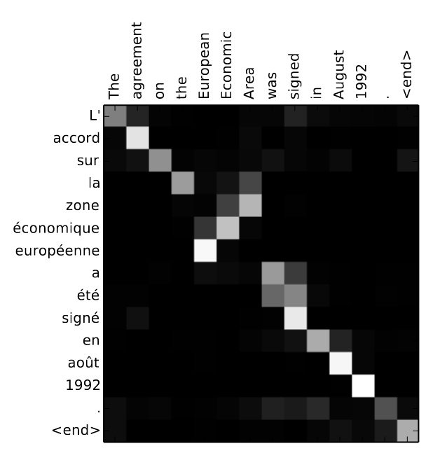
OK now we need to understand what the $e_{tk}$ are, but once we do, we are almost done — we’ll see all the dependencies, understand how the content vector is computed, and more importantly, grasp the whole point of the attention mechanism. The $e_{tk}$ are the alignment scores; a high score $e_{tk}$ indicates that the $t$th word in the translation is highly related to the $k$th word in the original, input sentence. We need to repeat, because this is truly the heart of the attention mechanism and what sets it apart from all previous approaches. A high alignment score $e_{tk}$ indicates that the $k$th word in the input sentence will have a high influence when deciding the $t$th word in the output sentence. This is precisely what we mean by dynamic weight allocation; we apply a different set of weights for each output word. Of course, the important question now is how the alignment scores $e_{tk}$ are computed.

Before we move on, it must be noted that we are now entering a point where attention mechanisms start to differentiate. In other words, what we explained up to this point seems to be fairly common across different attention approaches, but the rest of this section will provide some details specific to the approach of Bahdanau et al. The weights $e_{tk}$ are determined by using a learning-based approach; a standard, feed-forward network (an MLP) that uses the most recent decoder state and the $j$th state of the encoder: $$e_{tj} = a(s_{t-1}, h_j).$$ This makes sense; our goal is to find how the upcoming (i.e., $t$th) word in the translation is related to the $j$th word of the input sentence, and the MLP that we use compares the most recent decoder state with the $j$th encoder state. The MLP $a(\cdot)$ is trained jointly together with all other networks (i.e., the encoder and decoder RNNs).

It is worth doing a re-cap to see the entire structure of dependencies in the output

• The $t$th word $y_t$ depends on the decoder state $s_t$
• The state $s_t$ depends on the previous decoder state $s_{t-1}$, previous word $y_{t-1}$ and the current context vector $c_t$
• The context vector $c_t$ depends on all encoder states $\{h_j\}_j$ and weights $\{\alpha_{tj}\}_j$
• The weights $\{\alpha_{tj}\}_j$ depend on the alignment scores $\{e_{tj}\}_j$ for the $t$th word
• The alignment scores $\{e_{tj}\}_j$ depend on the most recent decoder state $s_{t-1}$ as well as all encoder states $\{h_j\}_j$.

The Transformer Model and its Attention Mechanism

While the approach of Bahdanau et al. uses MLP for determining the alignment scores, more recent approaches in fact use simpler strategies based on inner products. In particular, the Transformer model of Vaswani et al.^[5], which hugely boosted the popularity of attention mechanisms, relies on Scaled dot-product attention (Section 3.2.1). Before we move on, it is worth spending some time to make sure that we fully grasp the meaning of terms that are now standard, namely the Query, Key and Values — these terms need to be our second nature, otherwise we’ll have difficulty understanding the operations of the Transformed model.

Query, Key and Values

This terminology comes from the world of information retrieval (search engines, DB management etc.), where the goal is to find the values that match a given query by comparing the query with some keys. In the case of the attention mechanism, these terms can be thought of as below:

• Query: this is the entry for which we try to find some matches. For example, in the case of translation, the query is the entry that we use while translating the most recent word in a sentence. In the case of Bahdanau et al. above, this would be the hidden state vector $s_{t-1}.$ Just like when we make a Google or database search we have one query, so in this case we have one vector entry, $s_{t-1}$.
• Key: These are the entries that are matched against the query. That is, we compare all keys with the query, we quantify the similarity between each query-key pair. In the case of Bahdanau et al., the keys are the encoder hidden state vectors $h_1, h_2, \dots, h_T$. When we do a Google search, we match the query against ~all entries (i.e., keys) in the database. That is why our keys are all the hidden states; we are trying to fetch the states that are most relevant to the query.
• Value: The value $v_j$ is the entry corresponding to the $j$th key In the case of Bahdanau et al., it is once again the hidden state vectors $h_j$ that appear on the right hand side of the equation $$c_t = \sum\limits_{j=1}^{T_x} \alpha_{tj} h_j. $$ (See also Figure 16.5 in Rashka). Note that values are not the outputs — but outputs are weighted sums of the values.

As seen above, in the case of Bahdanau et al., the keys and values are of the same kind –they are the encoder’s hidden states $h_j$– but used for different purposes. When they are keys, they are used to quantify the similarity between the query and the decoder’s hidden states $s_{t-1}$, but when they are values they are the entries that we average over to produce the final context vector $c_t$. This does not need to be the case; keys and values can be different, as we’ll see in other examples of attention mechanisms.

In the remainder of the post, we’ll denote the query with $q_t$, the keys with $k_j$ and the values corresponding to each key with $v_j$.

The Transformer model relies on attention mechanisms on three distinct places. To see where, we first need to have a better understanding of the Transformer model.

The Transformer model is similar to the approach of Bahdanau et al. in that it also relies on an Encoder-Decoder architecture. The main difference is that the RNN’s of Bahdanau et al. are completely replaced with attention-based mechanisms. Hence the title of the paper of Vaswani et al.: “Attention is all you need”.

The encoder is responsible for taking the $n$ input words $x_1, \dots, x_n$ and producing an encoded representation for each word, $z_1, z_2, \dots, z_n$. Then, the decoder takes these encoded representations and produces the translated output. While producing each translated word $y_t$, the Transformer uses all the encoded words $z_1, z_2, \dots, z_n$ and all the words that have been produced up to the moment $t$.

The attention mechanisms are then used in three different places, with different query-key-value combinations (Section 3.2.3):

• Between the encoder and decoder. The query comes from the previous decoder layer and the keys come from the encoder layers.
• (Self-attention) Within the encoder, where all the keys, values and queries come from the same place, namely the output of the previous layer of the encoder. Each entry can attend to all positions.
• (Self-attention) Within the decoder, where all the keys, queries and entries come from the decoder layers but only up to the current position (to maintain the causality needed for the auto-regressive property).

Some more examples are helpful to further grasp the utility of these mechanisms. The attention between the encoder and the decoder is rather obvious, as we already discussed it with the network of Bahdanau et al.: The goal is to place higher emphasis on the input words that are more relevant to a particular output word. The second type is less obvious: Why do we need to apply self-attention between the input words? The examples in Figure 3 of Vaswani et al. are very helpful: The goal is to identify the words in the sentence that are related to one another.

More on self-attention

As we mention above, in the case of self-attention, the queries, keys and values all come from the same exact place. For example, they can be the hidden state of a word or they can even be the word itself. To take advantage of the learning that takes place in deep networks, we can always add some parameters that will be tuned from data. This is also a way to slightly differentiate between the queries, keys and values.

For example, if $x_i$ is the embedding or the hidden state vector of the $i$th word, then we can learn a simple query matrix, key and value matrices $U_q$, $U_v$ and $U_k$ that produce the query, key and matrix corresponding to this word as \begin{align}q_i &= U_q x_i \\ k_i &= U_k x_i \\ v_i &= U_v x_i \end{align}. Then, the alignment scores between the $i$th and the $j$th word can be computed as (sorry for the change of notation) $$\omega_{ij} = q_i^T k_j = x_i^T U_q^T U_k x_j.$$ This is still an inner product, but one that involves learned parameters for more flexibility. The context vector corresponding to the $i$th word is still computed using essentially the same formula above as $$c_i = \sum_j \alpha_{ij} v_j, $$ where $\alpha_{ij}$ is once again computed via softmaxing but also dividing by vector length $d_k$ (see last para of Section 3.2.1 of Vaswani et al.): $$\alpha_{ij} = \text{softmax}(\omega_{ij}/\sqrt{d_k})$$

References

1. Dzmitry Bahdanau and Kyunghyun Cho and Yoshua Bengio (2016): Neural Machine Translation by Jointly Learning to Align and Translate. 2016, (arXiv:1409.0473 [cs, stat]).
2. Ilya Sutskever and Oriol Vinyals and Quoc V Le (0000): Sequence to Sequence Learning with Neural Networks. In: 0000.
3. Kyunghyun Cho and Bart Merrienboer and Caglar Gulcehre and Dzmitry Bahdanau and Fethi Bougares and Holger Schwenk and Yoshua Bengio (2014): Learning Phrase Representations using RNN Encoder-Decoder for Statistical Machine Translation. 2014, (arXiv:1406.1078 [cs, stat]).
4. Dzmitry Bahdanau and Kyunghyun Cho and Yoshua Bengio (2016): Neural Machine Translation by Jointly Learning to Align and Translate. 2016, (arXiv:1409.0473 [cs, stat]).
5. Ashish Vaswani and Noam Shazeer and Niki Parmar and Jakob Uszkoreit and Llion Jones and Aidan N Gomez and Łukasz Kaiser and Illia Polosukhin (2017): Attention is all you need. In: Advances in neural information processing systems, vol. 30, 2017.